
United States
Description of cropping systems, climate, and soils
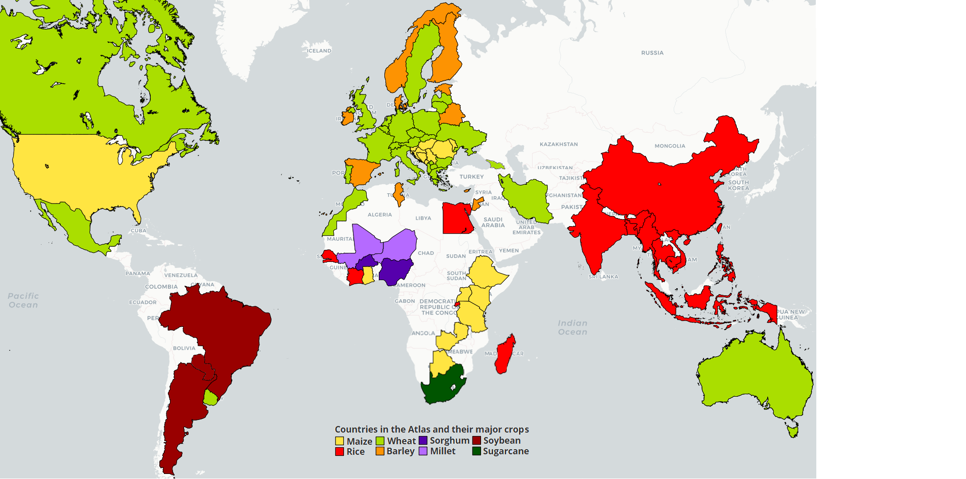
Annual crop production area in the United States of America (USA) occupies 97 million ha. Major crops are maize, soybean, wheat, and rice, which account for 87% of total crop area, and the country is one of the largest producers and exporters of these crops. During the last decade (2013-2022), the USA accounted for 27, 32, and 6% of global annual maize, soybean, and wheat productions, respectively. In turn, whereas rice area and production is relatively small compared with Asian countries, US is one of the major exporting countries of this crop.
Table 1. Average (2013-2022) total production, harvested area, and average yield of maize, soybean, wheat, and rice in USA. Source: FAOSTAT
| Crop | Total production (Mt) | Harvested area (M ha) | Average yield (t/ha) |
| Maize | 364.1 | 33.6 | 10.8 |
| Soybean | 111.2 | 33.6 | 3.3 |
| Wheat | 52.3 | 16.5 | 3.1 |
| Rice | 9.1 | 1.1 | 8.4 |
Maize-soybean crop systems
More than 85% of maize and soybean is produced in the north-central region known as the ‘Corn Belt’, where continuous maize (≈35%) and 2-year maize–soybean rotation (≈65%) are the dominant cropping systems. The central and eastern regions of the Corn Belt have favorable climate for rainfed crop production, with total annual rainfall that ranges from 800 to 1100 mm. The western edge of the Corn Belt has less rainfall and includes the eastern Great Plains states of North Dakota, South Dakota, Nebraska, and Kansas. Irrigated maize and soybean account for ca. 10-15% of the national production of these crops and their area concentrated in the western fringe of the region. Irrigated soybean is also produced along the Mississippi River valley (mainly in the state of Arkansas). In the Corn Belt, soils are generally deep, fertile, rich in organic matter, and have large water holding capacity in the rootable soil depth (i.e., > 200 mm plant available water). Dominant soils correspond to the Mollisols and Alfisols orders. A detailed description of weather, soil, and cropping systems can be found in Connor et al (2011) and Grassini et al. (2014). In wet years, transient early-season waterlogging is likely in soils with moderate-to-low infiltration rates in the central and eastern regions of the Corn Belt, where subsurface tile drainage is currently used on about one-third of total cropland to mitigate this problem (Sugg, 2007). In the past 60 years, there has been a shift from continuous maize under conventional tillage to a 2-year maize–soybean rotation under some form of conservation tillage (defined as any tillage method that leaves at least 30% of soil surface covered by plant residues). Of total area sown with maize and soybean, 52 and 75% is produced using conservation tillage, respectively (Horowitz et al., 2010). Almost all soybean area in the Corn Belt is sown with transgenic cultivars and the vast majority of those cultivars possess a transgene that provides tolerance to glyphosate. The use of glyphosate-resistant cultivars has provided near-total weed control (though glyphosate-resistant weeds are now increasingly appearing), and has accelerated producer adoption of conservation and no-tillage practices and narrower row spacing. Use of transgenic Bt maize with resistance to a number of damaging insect species is also widespread.
Wheat systems
There are three main wheat growing regions in the US, each with its own characteristic and growing different wheat classes. The Great Plains accounts for ~64% of US wheat production and is commonly divided into two regions: the northern (Montana, North Dakota, South Dakota, Wyoming and Nebraska) and southern Great Plains (Colorado, Kansas, Oklahoma, and Texas), accounting for ca. 33% and 31% of the wheat US production, respectively (USDA-NASS, 2015-2019). The southern Great Plains accounts for 57% of the total US winter wheat production and the most widely cultivated wheat class is high quality hard red winter wheat (USDA CDL 2017). The northern Great Plains represents 73% of the total US spring wheat production and the most widely cultivated wheat class is hard red spring wheat (USDA CDL 2017). In eastern US, about 2.3 Mha are sown to soft red winter wheat every year, which is a wheat class used for confectionary products like cookies and crackers. There are two additional minor wheat growing regions in the US, including the Pacific Northwest (hard red spring wheat and soft white winter wheat) and the Californa/Arizona desert (high quality durum wheat). This yield gap analysis focused on the northern and southern Great Plains, as well as the eastern U.S., which altogether account for 76% of US wheat harvested area.
Winter wheat is sown in autumn (Sep-Oct), reaching maturity in mid-summer (June-July) and spring wheat is sown early spring (Apr-May) and reaches maturity during late summer (Aug-Sep). There are strong latitudinal gradients for temperatures and longitudinal gradients for precipitation, elevation, and reference evapotranspiration in the southern Great Plains (Lollato et al., 2017). In comparison, the northern Great Plains have lower winter temperatures, which hamper winter wheat survival; and cooler summer temperatures, which allows for cultivation of spring wheat which goes through the reproductive stages during the summer. Due to the aforementioned weather gradients, the role of wheat within the cropping system changes considerably depending on the region within the US. In the central Kansas and north-central Oklahoma, wheat follows either soybean, maize, or a summer fallow (continuous wheat). Wheat following soybean has a delayed sowing and reduced yield potential (Staggenborg et al., 2003). Wheat following Maize or continuous wheat can be sown around the optimal time in this region, but is more exposed to Fusarium head blight and leaf spotting diseases. In western Kansas, Colorado, and the Oklahoma panhandle, wheat is grown following a long-term (14-month) fallow, a summer fallow, or continuously after maize (Peterson et al., 1996). These previous summer crops or fallow periods were simulated to account for the available water at sowing for the wheat crop. From central Oklahoma into Texas panhandle, about half of the winter wheat is grown as a dual-purpose crop, which is sown 3-4 weeks earlier than for grain-only using higher seeding rates, and grazed by cattle during the winter and early spring, usually yielding about 14% less than a grain-only wheat (Edwards et al., 2011). This system was not simulated as it would either require an animal growth and development model or include coarse assumptions. While the production system is much more diverse in the northern Great Plains, especially in North Dakota, the spring wheat is sown after a winter fallow and therefore we did not simulate a previous summer crop, only simulating the soil water dynamics during the preceding fallow. In Ohio, winter wheat is mainly cultivated in rotation with soybean.
Rice crop systems
U.S. rice production can be split into three ecological zones, the Upper Sacramento Valley (CA), the Gulf Coast (TX, LA, and parts of MS), and the Mississippi River Valley (AR, MO, and parts of MS) (Livezey and Foreman, 2004). Although each of these regions has unique climate characteristics, the climate in the two Southern regions is generally humid with a small range of diurnal temperature variation compared to the climate in CA, which is generally arid/semiarid with large diurnal temperature variation. CA growers use primarily medium-grain temperate japonica rice varieties, whereas growers in the Southern regions primarily use long-grain tropical japonica and hybrid rice varieties. The use of hybrids and herbicide resistant varieties is increasing in the Southern U.S. since roughly 2001, while CA still uses primarily conventional inbred varieties. U.S. rice production systems are direct seeded; CA rice is primarily water-seeded (i.e. – pre-soaked seed is applied to flooded fields via airplane), whereas Southern U.S. rice is primarily drill-seeded. Furthermore, in the southern U.S., rice systems are often rotated with other crops (i.e. soybean and maize) while in CA, due to poorly drained heavy clay soils not suitable for other crops, most rice systems are continuous rice.
Data sources and assumptions
Harvested area and actual yields
The SPAM harvested area maps were used for selecting the reference weather stations for each crop and water regime case. County-level data on crop harvested area and average yields for each crop were retrieved from the USDA-NASS quick stats (http://www.nass.usda.gov/Quick_Stats/). Statistics from 10 cropping seasons were used to calculate average yields for maize (2013-2022), for soybean and wheat (2009-2018) and from five cropping seasons (2010-2014) for rice.
Weather data and reference weather stations
For rainfed and irrigated maize and soybean, historical (last 20+ years) measured daily weather data, including solar radiation, maximum and minimum air temperature, precipitation, relative humidity and wind speed were obtained from the High Plains Regional Climate Center (HPRCC), the Illinois Water and Atmospheric Resources Monitoring Program (WARM), Ohio Agricultural Research and Development Center (OARDC) Weather Service, the University of Wisconsin Extension Ag Weather, the Indiana Purdue Automated Agricultural Weather Station Network (PAAWS), North Dakota Agricultural Weather Network (NDAWN), Michigan State University Enviro-Weather, Oklahoma Mesonet, State Climate Office of North Carolina (SCO), West Texas Mesonet, the University of Minnesota Southern and Southwest Research and Outreach Centers, the South Dakota Climate and Weather, the Missouri Mesonet (AgEBB), the Texas A&M Integrated Agricultural Information and Management System (iAIMS) Climatic Database†, and ten weather stations in NC, SD, TX, and WI reported through the National Oceanic and Atmospheric Administration (NOAA). Meteorological stations selected from these networks are located in agricultural areas, rather than in urban areas, which helps to ensure the representativeness of the weather data for estimating yield potential.
For wheat, historical (last 20+ years) measured daily weather data, including solar radiation, maximum and minimum air temperature, precipitation, relative humidity were obtained from the High Plains Regional Climate Center (HPRCC), North Dakota Agricultural Weather Network (NDAWN), Montana Mesonet, Oklahoma Mesonet, Colorado Mesomet, and the Texas A&M Integrated Agricultural Information and Management System (iAIMS) Climatic Database. Similar to maize and soybean, these stations are located in primarily agricultural rather than urban areas.
For irrigated rice, historical (last 13 to 15 years) measured daily weather data included maximum and minimum air temperature, precipitation, relative humidity, and wind speed. Data were retrieved from the California Irrigation Management Information System (CIMIS), the National Weather Service (NWS) station network, the Louisiana Agriclimatic Information System, the Delta Agricultural Weather Center, and the Texas A&M Integrated Agricultural Information and Management System (iAIMS) Climatic Database. Similar to maize, soybean, and wheat, these stations are located in primarily agricultural rather than urban areas.
Quality control and filling/correction of the weather data was performed based on GYGA weather protocols and comparison against weather records from adjacent National Weather Service-Cooperative Observer Network (NWS-COOP) meteorological stations. We used gridded daily data from the NASA Prediction of Worldwide Energy Resource (POWER; http://power.larc.nasa.gov/) to fill missing solar radiation data and, for eight maize weather stations, as source of relative humidity and wind speed data. Moreover, for maize, for those stations that do not measure solid precipitation (snow), but snow contribution might still be important to recharge the soil profile during fallow, missing winter/early spring precipitation values were filled with data from their closest NOAA weather station measuring snow, which were located between 0.5 and 40 km away (average distance = 8 km). Only 25% of the snow was assumed to infiltrate the soil (Grassini et al., 2010). Hence, complete long-term weather records were available for simulating yield potential (Yp) for irrigated crops and water-limited yield potential (Yw) for rainfed crops.
Based on crop harvested area distribution and the agro-climatic zones defined for the USA (Van Wart et al., 2013a), a total of 20 and 45 reference weather stations (RWS) were selected for irrigated and rainfed maize, while a respective 14 and 41 RWSs were selected for irrigated and rainfed soybean, following van Bussel et al (2015). A total of 35 RWS were selected for wheat and 14 for rice. RWS buffer zones accounted for 55 and 61% of total harvested area for irrigated and rainfed maize, 56 and 55% of total harvested area for irrigated and rainfed soybean, 43% for rainfed wheat and 87% for irrigated rice. The agro-climatic zones where these locations were located accounted for 72, 87, 73, 77, 61% and 92% of national area for these crop-water regimes combinations.
Soil data
For rainfed crops, the dominant soil series were identified for each RWS buffer based on gSSURGO soil database (NRCS, Soil Survey Staff). Briefly, maize and soybean harvested area within each soil type within each RWS buffer was calculated and we included as many soil types as needed to cover ≥50% maize and soybean area within each buffer. Rooting depth was set at 1.5 m for all soil types due to the lack of physical and chemical constrains to root growth and based on observed soil water extraction patterns for maize and soybean (Payero et al., 2006; Ordoñez et al., 2018).
Crop system and management information for crop simulations
Maize simulations
Management practices were obtained for each RWS buffer zone. Average sowing date was retrieved from USDA-RMA, while data on cultivar maturity were provided by seed companies and local agronomists. Requested information include: dominant crop rotations and proportion of each of them to the total harvested area, average sowing dates, dominant cultivar name and maturity, and actual and optimal plant population density. The provided data were subsequently corroborated by other local and national experts. Further details on management input data can be found in Morell et al. (2016).
Simulations using maturity of the most widely used cultivar for the region surrounding each RWS were performed using Hybrid-Maize model (Yang et al., 2004). The model was previously validated for its ability to simulate maize yield potential across a wide range of environments in the Corn Belt (Grassini et al., 2009; Liu et al., 2005) and found to be robust at portraying key G x E x M interactions across a wide range of yields, ranging from 0.5 to 18 Mg ha-1. The model does not require site-specific parameter calibration for simulating yield potential, that is, all model parameters governing photosynthesis, respiration, leaf area expansion, light interception, biomass partitioning, and grain filling rate and duration are generic (Yang et al., 2004). To portray accurately the phenological development of new cultivars, model genetic coefficients were calibrated based on a relationship between hybrid relative maturity and duration of vegetative (emergence to silking) and reproductive phases (silking to blacklayer), expressed in growing degree days, derived from data collected from field experiments conducted in Ames, IA (Archontoulis et al., unpublished data). These experiments included 25 modern hybrids from the two most popular maize seed companies, with relative maturities ranging from 72 to 120 days.
To account for differences in initial soil water at sowing time among years, simulations of rainfed crops were initiated at immediately after harvest of the prior crop assuming 75% of plant available soil water based on Grassini et al. (2009). Soil surface residue coverage at harvest of the prior crop was set at 50% to reflect the large amount of non-grain aboveground biomass left by previous crop and the large proportion of maize production area under no-till or conservation tillage practices (Horowitz et al., 2010). Surface runoff was assumed negligible to reflect producer preference for avoiding highly sloping land for maize production, and wide adoption of conservation tillage and no-till practices, which greatly reduce runoff. Because dominant crop rotations are 2-y soybean-maize and continuous maize, maize yield potential was simulated for all the years for which weather data were available. Because there is little (if any) difference between actual and optimal plant population, the simulations were based on the range of optimal plant population reported for each buffer zone by the local agronomists. Simulations assumed no limitations to crop growth by nutrients and no yield reductions due to weeds, pests, and diseases.
A factor that is not accounted for by the crop simulation model, with a likely positive impact on rainfed yields (especially in drought years), is the water supply from perched water tables in the central and eastern regions of the Corn Belt. Five independent sources of information were used to identify RWS buffers with likely influence of perched water tables on water-limited yields: (i) data on depth to water table from gSSURGO (NRCS Soil Survey Staff), (ii) maps on subsurface tile-drained area distribution in USA (Sugg, 2007; Rizzo et al., 2018; Mourtzinis et al., 2021, (iii) consultation with local agronomists, (iv) data from shallow groundwater wells networks (e.g., http://isws.illinois.edu/warm/groundwater/), and (iv) trends in actual yield at these locations (i.e., high yields with little year-to-year variation despite contrasting differences in rainfall). Following this approach, we identified 33 RWS buffer zones in the central and eastern regions of the Corn Belt where “sub-surface irrigation” is very likely to have a positive impact on rainfed fields. We assumed that water was non-limiting for those fields located in areas with presence of water table within the rootable soil depth during the growing season. At these 33 RWS, separate simulations were performed for water-limited (no influence of water table) and non-water limited environments (soils with water table within the rootable soil depth during the maize growing season) and results were weighted based on their relative share of maize harvested area. In the case of irrigated crops in the southern Great Plains (OK, TX and southeastern KS), maximum temperature during the peak of the growing season was reduced by 0.5ºC to account for the ‘cooling’ effect associated with frequent irrigations in this region.
Simulations utilized weather, soil, and management data obtained for each RWS. For each RWS, all selected soil types were simulated and then weighted by their relative proportion to retrieve an average Yw at the level of the RWS buffer zone. Quality control of results was performed following the guidelines provided by Grassini et al. (2015).
A weighted average actual yield was calculated separately for rainfed and irrigated crops based on the actual yield reported by USDA-NASS quick stats, considering the proportion of each county that fall within each buffer zone and their relative contribution to the total crop harvested area in the buffer zone. Unfortunately, USDA-NASS county-level statistics stopped discerning between rainfed and irrigated areas and yields in recent years for most regions. In those county-year combinations where maize area and actual yields were not disaggregated by water regime but irrigation may still be important, a tier approach was used to estimate rainfed and irrigated areas and yields. When missing, the fraction of a county maize area under irrigation was (i) retrieved from the 2017 USDA Census of Agriculture, (ii) assumed equal to previous year’s average, (iii) computed with SPAM. Missing actual yields for irrigated maize were assumed equal to (i) the county average if the fraction of maize area under irrigation was greater than 80%, (ii) assumed equal to the average irrigated yield of its corresponding agricultural district, when reported, (iii) or assumed equal to previous years irrigated yield average. Missing actual yields for rainfed maize in counties with more than 10% of irrigation were computed by penalizing the average yield of the county by a factor that relates the county rainfed yield with the overall county average yield, which was computed using data from previous years for the same county or buffer. There were, at least, 5 counties within each RWS buffer (average of 10 counties per RWS). Reported Yw and Yp in the Global Yield Gap Atlas are long-term (20+ years) averages. In some county-year combinations, an important fraction of the planted maize area was not harvested due to severe droughts. Hence, we recalculated the average yield of rainfed maize in those cases by considering the ratio between the area planted with maize and the harvested. Yield gap (Yg) was calculated as the difference between long-term average Yw or Yp (2000-2022) and average actual farmers' yields (2013-2022).
Soybean simulations
Management practices were obtained for each RWS buffer zone. In the Corn Belt, sowing date, cultivar maturity group, and seeding rate were obtained from a large producer dataset including management data from more than 8,000 fields sown with soybean during the 2014-2017 cropping seasons (Rattalino Edreira et al., 2017). Late sowing date is a major cause for soybean yield gap in the US North Central region; hence, we derived the sowing date for our simulations from the 5th percentile of the sowing date distribution in each buffer, which typically corresponded to late-April and early-May sowing. Using average sowing date would have led to an underestimation of the yield potential and yield gap. For irrigated soybean in the state of Arkansas, we used the recommended sowing date and cultivar maturity group to maximize the yield potential for full-season irrigated systems (Salmerón et al., 2016). In the Mississippi river valley, we excluded double cropping system as it represents < 15% of the irrigated soybean harvested area (USDA NASS, 2004-2008 period).
Simulations using maturity of the most widely grown maturity group for the region surrounding each RWS were performed using APSIM soybean (v7.9) model (Holzworth et al., 2014). The model was previously validated for its ability to simulate soybean yield potential across a wide range of environments in the U.S. Corn Belt (Archontoulis et al., 2014, 2020, Ebrahimi-Mollabashi et al., 2019, Martinez-Feria et al., 2018) and found to be robust at portraying key G x E x M interactions across a wide range of yields, from 1.5 to 6.5 Mg ha-1. The model has a set of generic maturity groups (from MG 00 to MG 9, increments every 0.5 group) similarly to hybrid-maize model, which means minimum input requirements by the user. For details on the generic cultivars we refer to Archontoulis et al., (2014). We set up APSIM soybean to simulate a water-limited production situation. We used the SoilWat water balance model (typing bucket, Prober et al., 1998). Crop roots allowed to grow up to 1.5 m, which is the average max soy depth in the central US Corn Belt (Ordonez et al., 2018; Nichols et al., 2019). Soil water hydrological parameters developed by using texture class, plant available water, and Saxton and Rawls (2006) pedotransfer equations. To account for differences in initial soil water at planting time among years, simulations of rainfed crops were initiated on Jan 1 assuming 100% of plant available soil water. In APSIM, the soil water balance typically reaches equilibrium within 2-3 months. Previous crop residue on Jan 1 was assumed to be maize (amount 4 t dry matter /ha). The impact of water table on yields was accounted for similar as for the maize simulations. Briefly, we assumed that water was non-limiting for those fields located in areas with presence of water table within the rootable soil depth during the growing season. For the RWS with presence of water table, separate simulations were performed for water-limited (no influence of water table) and non-water limited environments (soils with water table within the rootable soil depth during the maize growing season) and results were weighted based on their relative share of maize harvested area.
Soybean yield potential was simulated for all the years for which weather data was available, assuming no limitations to crop growth by nutrients. For each RWS, all selected soil types were simulated and then weighted by their relative proportion to retrieve an average Yw at the level of the RWS buffer zone. A weighted average actual yield was calculated based on the actual yield reported, separately for rainfed and irrigated crops, for the counties that coincided with the buffer zone and the relative contribution of each county to the total crop harvested area in the buffer zone. There were, at least, 5 counties within each RWS buffer (average of 10 counties per RWS). Reported Yw and Yp in the Atlas are long-term (20+ years) averages.
Yield gap (Yg) was calculated as the difference between long-term average Yw or Yp and average (2009-2018) actual farmers' yields. Including more years before 2009 in the calculation of average actual yield would bias the estimate of average actual yield due to a strong, upward technology trend in the USA. Similar to maize, the Yp and Yw for some locations in the northern fringe of the region was relatively low and the resulting Yg small. We suspect that potential yields are higher than the current model predicts, possible because the current trigger for a leaf senescence as a result of cold damage is too conservative.
Wheat simulations
Management practices were obtained for each RWS buffer zone. Average sowing date was retrieved from extension bulletins, variety performance trials, and local agronomists. Requested information included: dominant crop rotations and proportion of each of them to the total harvested area, average sowing dates, actual and optimal plant population density. The provided data were subsequently corroborated by other national experts.
Simulations using maturity of the most widely used cultivar for the region surrounding each RWS were performed using SSM Wheat (Soltani and Sinclair, 2012). The model was previously validated for its ability to simulate hard red winter wheat phenology and yield potential across a wide range of environments in the US southern Great Plains (Lollato et al., 2017; 2019) and found to be robust at portraying key G x E x M interactions across a wide range of yields derived from 45 environments, ranging from 1.5 to 8.5 Mg ha-1. The calibration and validation of the SSM Wheat model for phenology and yield potential of other wheat types in different regions (i.e., hard red spring wheat in the US northern Great Plains, and soft red winter wheat in eastern US) occurred against data from intensively managed wheat trials (Shawn Conley, personal communication; Quinn and Steinke, 2019) and variety performance tests. For hard red spring wheat, the yield range in the 21 site-years validation dataset was 1.32-7.33 Mg ha-1, and for soft red winter wheat it was 2.76-12.1 Mg ha-1 across 23 site-years. Model validation indicated an overall a root mean square error below 5% for phenology and below 20% for grain yield.
We set up SSM Wheat to simulate a water-limited production situation. Crop roots were allowed to grow up to 1.5 m, which is the average max wheat depth in the central US Great Plains (Awad et al. 2018). Soil water hydrological parameters were derived from Saxton and Rawls (2006) pedotransfer equations. To account for differences in initial soil water at planting time among years, either the growth and development of the previous crop (i.e., wheat, corn, or soybeans) was simulated and the soil water content at crop maturity was used as initial soil water content for the wheat crop; or the soil water dynamics during the preceding fallow period (~15-d when following corn, ~3-m when following wheat, or 14-month duration) was simulated. In both cases, the SSM model was used for simulating the water balance.
Wheat yield potential was simulated for all the years for which weather data were available, assuming no limitations to crop growth by nutrients. For each RWS, all selected soil types were simulated and then weighted by their relative proportion to retrieve an average Yw at the level of the RWS buffer zone. Spring wheat and winter wheat were simulated separately for two stations in Montana, which included both type of wheat, and their results were weighted in each buffer using the harvest area proportion of spring over winter wheat (USDA CDL 2017). Similarly, a weighted average actual yield was calculated based on the actual yield reported (separately for spring and winter wheat) for the counties that coincided with the buffer zone and the relative contribution of each county to the total crop harvested area in the buffer zone. There were, at least, 5 counties within each RWS buffer (average of 10 counties per RWS). Reported Yw and Yp in the Atlas are long-term (20+ years) averages. Yield gap (Yg) was calculated as the difference between long-term average Yw or Yp and average (2009-2018) actual farmers' yields.
Rice simulations
Yield potential was estimated by simulation using the ORYZA (v3) crop model (Bouman et al., 2001). This model was chosen due to its widespread use and existing body of work validating it for various rice cropping systems. Further calibration and validation of this model was required to adequately simulate rice yield potential for representative high-yielding varieties typical of the types most widely planted in major U.S. rice-producing regions as described in Espe et al. (2016). In order to minimize the effect of variation between simulations, yield potential was simulated for each buffer zone over a 15-year time span at all locations except those in LA, which only had 13 years of weather data. Long-term mean yield potential in RWS buffer zones and as aggregated for larger spatial scales followed GYGA procedures.
For each buffer zone, the average emergence date as reported by state agronomists was used to initiate simulations. Sensitivity analyses were performed to evaluate the impact of using the long-term average emergence date rather than a distribution of emergence dates centered at the average, with only slight yield differences observed (absolute difference of less than 0.25 Mg ha-1; results not presented). Therefore, the average emergence date was deemed suitable for simulating yield potential. Annual simulated yield potentials were then averaged by buffer zone to determine the buffer zone yield potential. Individual simulation results were quality controlled for unrealistic results or failed simulations prior to averaging.
Data from the USDA-NASS database (USDA - National Agricultural Statistics Service, 2016) were used to determine actual yields within each buffer zone. Since buffer zones were constructed without regard for state or county boundaries, county-level data were retrieved and aggregated to obtain estimates for each buffer zone. In order to do this, the buffer zone average yield was calculated as a weighted average of county estimates, where weights were determined by the proportion of buffer zone harvested area within each county.

Where Yk is the average yield for buffer zone k, µj is the average reported yield for county j, n is the number of counties with harvested acres in buffer zone k, aj is the harvested area of county j in buffer zone k, and ak is the total harvested area in buffer zone k. To minimize potential confounding effects of yield trends over time, only the most recent reported data (2010 to 2014) was used. Buffer zone estimates were calculated by year and then averaged across years to get the average buffer zone yield.
† We thank Dennis Todey (South Dakota State University), Ken Scheeringa (Purdue University), Rick Wayne (University of Wisconsin-Madison), Mark Seeley (University of Minnesota), Jenny Atkins (WARM Program, University of Illinois at Urbana-Champaign), Daryl Herzmann (Iowa State University), and Bill Sorensen and Natalie Umphlett (UNL) for their help to access historical daily weather data.
References:
Archontoulis SV, Miguez FE, Moore KJ, 2014. A methodology and an optimization code to calibrate phenology of short-day species included in the APSIM PLANT model: application to soybean. Environmental Modeling and Software 62: 465–477.
Archontoulis SV, Castellano MJ, Licht MA, Nichols V, Baum M, Huber I, Martinez-Feria R, Puntel L, Ordóñez RA, Iqbal J, Wright EE, Dietzel RN, Helmers M, Vanloocke A, Liebman M, Hatfield JL, Herzmann D, Córdova SC, Edmonds P, Togliatti K, Kessler A, Danalatos G, Pasley H, Pederson C, Lamkey KR, 2020. Predicting Crop Yields and Soil-Plant Nitrogen Dynamics in the US Corn Belt. Crop Science, 1–18.
Awad, W., Byrne, P.F., Reid, S.D., Comas, L.H. and Haley, S.D., 2018. Great plains winter wheat varies for root length and diameter under drought stress. Agronomy Journal, 110(1), 226-235.
Bouman, B., Kropff, M., Tuong, T., Wopereis, M., ten Berge, H., van Laar, H., 2001. Oryza2000: modeling lowland rice, ed. International Rice Research Institute.
Connor, D.J., Loomis, R.S., Cassman, K.G., 2011. Crop Ecology. Productivity and Management in Agricultural Systems. Cambridge Univ. Press, Cambridge, UK.
Edwards, J.T., Carver, B.F., Horn, G.W. and Payton, M.E., 2011. Impact of dual‐purpose management on wheat grain yield. Crop Science, 51(5), 2181-2185.
Espe, M.B., Yang, H., Cassman, K.G., Guilpart, N., Sharifi, H., Linquist, B.A., 2016. Estimating yield potential in temperate high-yielding, direct-seeded US rice production systems. F. Crop. Res. In press. doi:10.1016/j.fcr.2016.04.003
Food and Agriculture Organization of the United Nations, FAO Statistical Databases. 747 Available at http://faostat.fao.org/
Grassini, P., Specht, J.E., Tollenaar, M., Ciampitti, I., Cassman, K.G., 2014. High-yield maize–soybean cropping systems in the US Corn Belt. In: Crop Physiology (2nd Edition), Sadras, V.O., Calderini, D.F. (Eds). Academic Press, San Diego.
Grassini, P., van Bussel, L.G.J, Van Wart, J., Wolf, J., Claessens, L., Yang, H., Boogaard, H., de Groot, H., van Ittersum, M.K., Cassman, K.G., 2015. How good is good enough? Data requirements for reliable crop yield simulations and yield-gap analysis. Field Crops Res. 177, 49-63.
Grassini, P., Yang, H., Cassman, K.G., 2009. Limits to maize productivity in Western Corn-Belt: A simulation analysis for fully irrigated and rainfed conditions. Agric. Forest 761 Meteoro. 149, 1254-1265.
Grassini, P., You, J., Hubbard, K. G., & Cassman, K. G. (2010). Soil water recharge in a semi-arid temperate climate of the Central US Great Plains. Agricultural Water Management, 97(7), 1063-1069.
Holzworth, D. P., Huth, N. I., deVoil, P. G., Zurcher, E. J., Herrmann, N. I., McLean, G., … Keating, B. A., 2014. APSIM-evolution towards a new generation of agricultural systems simulation. Environmental Modelling & Software, 62, 327–350.
Horowitz, J., Ebel, R., Ueda, K., 2010. No-till farming is a growing practice. USDA-ERS Economic Information Bulletin No. 70.
Ebrahimi-Mollabashi E, Huth NI, Holzwoth DP, Ordonez RS, Hatfield JL, Huber I, Castellano MJ, Archontoulis SV, 2019. Enhancing APSIM to simulate excessive moisture effects on root growth. Field Crops Research 236: 58–67.
Fischer, R.A., 2015. Definitions and determination of crop yield, yield gaps, and of rates of change. F. Crop. Res. 182, 9–18. doi:10.1016/j.fcr.2014.12.006
Liu, X., Andresen, J., Yang, H., and Niyogi, D., 2015. Calibration and Validation of the Hybrid-Maize crop model for regional analysis and application over the U.S. Corn Belt. 802 Earth Interactions. 19, 1-16.
Livezey, J. and L. Foreman. 2004. Characteristics and production costs of U.S. rice farms. US Dept. of Ag. Statistical Bulletin. 974-7.
Lobell, D.B., Cassman, K.G., Field, C.B., 2009. Crop Yield Gaps: Their Importance, Magnitudes, and Causes. Annu. Rev. Environ. Resour. 34, 179–204. doi:10.1146/annurev.environ.041008.093740
Lollato, R.P., Edwards, J.T., Ochsner, T.E., 2017. Meteorological limits to winter wheat productivity in the U . S . southern Great Plains. F. Crop. Res. 203, 212–226. https://doi.org/10.1016/j.fcr.2016.12.014
Lollato, R.P., Ruiz Diaz, D.A., DeWolf, E., Knapp, M., Peterson, D.E. and Fritz, A.K., 2019. Agronomic practices for reducing wheat yield gaps: a quantitative appraisal of progressive producers. Crop Science, 59(1), 333-350.
Martinez-Feria R; Castellano M; Dietzel R; Helmers M; Liebman M; Huber I; Archontoulis SV, 2018. Linking crop- and soil-based approaches to evaluate system nitrogen-use efficiency and tradeoffs. Agriculture, Ecosystems and Environment 256: 131-143
Morell FJ, Yang HS, Cassman KG, Van Wart J, Elmore RW, Licht M, Coulter JA, Ciampitti IA, Pittelkow CM, Brouder SM, Thomison P, Lauer J, Graham C, Massey R, Grassini P (2016) Can crop simulation models be used to predict local to regional maize yields and total production in the U.S. Corn Belt? Field Crops Research (In Press) doi 10.1016/j.fcr.2016.04.004
Mourtzinis, S., Andrade, J.F., Grassini, P., Edreira, J.I.R., Kandel, H., Naeve, S., Nelson, K.A., Helmers, M. and Conley, S.P., 2021. Assessing benefits of artificial drainage on soybean yield in the North Central US region. Agricultural Water Management, 243, p.106425.
Nichols, V., Ordóñez, R. A., Castellano, M. J., Liebman, M., Hatfield, J. L., Helmers, M., … Archontoulis, S. V. (2019). Vertical distribution of maize and soybean roots in Iowa, USA. Plant and Soil, 444, 225–238
Ordóñez, R.A., Castellano, M.J., Hatfield, J.L., Helmers, M.J., Licht, M.A., Liebman, M., Dietzel, R., Martinez-Feria, R., Iqbal, J., Puntel, L.A., Córdova, S.C., Togliatti, K., Wright, E.E., Archontoulis, S.V., 2018. Maize and soybean root front velocity and maximum depth in Iowa, USA. Field Crops Res. 215, 122-131.
Payero, J.O., Klocke, N.L., Schneekloth, J.P., Davison, D.R., 2006. Comparison of irrigation strategies for surface-irrigated corn in West Central Nebraska. Irrig. Sci. 24, 817 257-265.
Peterson, G.A., Schlegel, A.J., Tanaka, D.L. and Jones, O.R., 1996. Precipitation use efficiency as affected by cropping and tillage systems. Journal of Production Agriculture, 9(2), 180-186.
Probert, M. E., Dimes, J. P., Keating, B. A., Dalal, R. C., & Strong, W. M. (1998). APSIM’s water and nitrogen modules and simulation of the dynamics of water and nitrogen in fallow systems. Agricultural Systems, 56, 1–28.
Quinn, D., and K. Steinke. 2019. Soft Red and White Winter Wheat Response to Input‐Intensive Management. Agronomy Journal 111, no. 1: 428-439.
Rattalino Edreira, J.I., Mourtzinis, S., Conley, S.P., Roth, A.C., Ciampitti, I.A., Licht, M., Kandel, H., Kyveryga, P.M., Lindsey, L.E., Mueller, D.S., Naeve, S.L., Nafziger, E., Specht, J.E., Stanley, J., Staton, M.J., Grassini, P., 2017. Assessing causes of yield gaps in agricultural areas with diversity in climate and soils. Agric. For. Meteorol. 247, 170-180.
Rizzo, G., Edreira, J.I.R., Archontoulis, S.V., Yang, H.S. and Grassini, P., 2018. Do shallow water tables contribute to high and stable maize yields in the US Corn Belt?. Global food security, 18, pp.27-34.
Salmerón, M., Gbur, E.E., Bourland, F.M., Buehring, N.W., Earnest, L., Fritschi, F.B., Golden, B.R., Hathcoat, D., Lofton, J., McClure, A.T., Miller, T.D., Neely, C., Shannon, G., Udeigwe, T.K., Verbree, D.A., Vories, E.D., Wiebold, W.J., Purcell, L.C., 2016. Yield response to planting date among soybean maturity groups for irrigated production in the US Midsouth. Crop Sci. 56, 747–759.
Soltani, A., Sinclair, T.R., 2012. Modeling Physiology of Crop Development, Growth and Yield. CAB International, Cambridge, MA.
Soil Survey Staff, Natural Resources Conservation Service, United States Department of Agriculture. Web Soil Survey. Available online at http://websoilsurvey.nrcs.usda.gov/
Soltani, A., Sinclair, T.R., 2012. Modeling Physiology of Crop Development, Growth and Yield. CAB International, Cambridge, MA.
Sugg, Z., 2007. Assessing U.S. farm drainage: can GIS lead to better estimates of subsurface drainage extent? World Resources Institute, Washington D.C [online WWW]. Available URL:http://pdf.wri.org/assessing_farm_drainage.pdf
Staggenborg, S.A., Whitney, D.A., Fjell, D.L. and Shroyer, J.P., 2003. Seeding and nitrogen rates required to optimize winter wheat yields following grain sorghum and soybean. Agronomy Journal, 95(2), 253-259.
USDA–National Agricultural Statistics Service (NASS), 2000-2014. Quick stats 2.0. 843 Available at: http://quickstats.nass.usda.gov/
van Bussel, L.G.J., Grassini, P., Van Wart, J., Wolf, J., Claessens, L., Yang, H., Boogaard, H., de Groot, H., Saito, K., Cassman, K.G., Van Ittersum, M.K., 2015. From field to atlas: Upscaling of location-specific yield gap estimates. Field Crops Res, 117, 853 98-108.
Water and Atmospheric Resources Monitoring Program. Shallow Groundwater Network. (2015). Illinois State Water Survey, 2204 Griffith Drive, Champaign, IL 61820-7495. http://dx.doi.org/10.13012/J8CC0XMK
Van Wart, J., Van Bussel, L.G.J., Wolf, J., Licker, R., Grassini, P., Nelson, A., Boogaard, H., Gerber, J., Mueller, N.D., Claessens, L., Cassman, K.G., Van Ittersum, M.K., 2013a. Reviewing the use of agro-climatic zones to upscale simulated crop yield potential. Field Crops Res. 143, 44-55.
Yang, H.S., Dobermann, A., Lindquist, J.L., Walters, D.T., Arkebauer, T.J., Cassman, K.G., 2004. Hybrid-maize - A maize simulation model that combines two crop modeling 882 approaches. Field Crops Res. 87, 131-154.
Get access to the Atlas for advanced users
Download GYGA results
| Please read the license information in case you are interested in using the data from the Global Yield Gap Atlas. | |
| read more>> |
 Country agronomists
Soybean team:
|
Sotirios Archontoulis |
Shawn Conley |


Wheat team:
|
Romulo Lollato |
Joel Ransom |
|
Laura Lindsey |
|


Maize team:
|
Chris Graham |
Cameron Pittelkow |
|
Peter Thomison |
Sylvie Brouder |
|
Raymond Massey |
Jeff Coulter |
|
Joe Lauer |
Mark Licht |
|
Ignacio Ciampitti |


Rice team:
|
Bruce A. Linquist Dept. of Plant Sciences, University of California - Davis, Davis, CA, USA |
Matthew B. Espe Dept. of Plant Sciences, University of California - Davis, Davis, CA, USA |
|
Dustin Harrell LSU AgCenter, College of Agriculture, Louisiana State University, Baton Rouge, LA, USA |
Steve Linscombe LSU AgCenter, College of Agriculture, Louisiana State University, Baton Rouge, LA, USA |
|
Kent McKenzie Rice Experiment Station, California Cooperative Rice Research Foundation, Biggs, CA, USA |
|


Merle Anders
Net-Profit Crop Consultancy PLLC, AR, USA
Donn Beighley
Dept. of Agriculture, Southeast Missouri State University, Malden, MO, USA
Randall Mutters
University of California Cooperative Extension, Oroville, CA, USA
Ted Wilson
Texas A&M AgriLife Research Center, Beaumont, TX, USA