
 GYGA Protocol for Model Calibration
Crop simulation models: selection, calibration, use, and quality control of simulated yields
1. MODEL SELECTION
Desirable attributes of crop simulation models are summarized by van Ittersum et al. (2013) and shown in Appendix I. We argue that rather than using a single generic model globally, it is more important that a particular model has been calibrated and evaluated for the conditions to be simulated. Thus, models may differ per region or crop, as long as the models have been validated under those conditions. Preferably, the same model will be used for the same crop to simulate Yw and Yp at locations within the same countries or geographic region such as Sub-Saharan Africa or North America.
2. MODEL CALIBRATION
Different crop cultivars are planted across locations, hence, it is necessary to calibrate crop models to account for difference in crop phenology and growth-related factors. Simulations will aim to portray most recently released high-yield crop cultivars, grown in pure stands. The following preference list will be followed to determine the preferable source of data for model calibration:
- Elaborate calibration: this requires field experiments where crops were grown without evident nutrient limitations and no incidence of biotic adversities and where all weather, soil, and management data required to run the field-year specific simulation are available (see Appendix II and III for the data requirements and procedure for a complete model calibration). If such experiments are not available for a specific country or region within a country, we may use crop growth data from experiments in which crops are grown with optimal management for very similar regions in terms of climate and soils—hopefully from the same climate zone (Van Wart et al., 2013a).
- Simple (only phenology) calibration: if (1) is not possible, use the methodology in van Wart et al (2013b) to calibrate the simulated crop phenology for each crop-buffer zone. Briefly, we proposed to optimize model coefficients (related to phenology) until the simulated physiological maturity matches the actual physiological maturity date (or harvest date – see Appendix IV) reported by the country agronomist. This phenology calibration is preferably done based on the buffer-specific weather data and sowing and maturity dates specified by the country agronomist. In those countries or regions where calculated sowing-to-maturity growing-degree days (GDD) vary little among crop-buffer zones (CV=5%), the same GDD value will be used for all crop-buffer zones. This should also be followed by a calibration of the flowering dates. If actual flowering dates are not reported by country agronomists, it can be determined using generic rules (for example, in maize the GDD before and after silking are typically the same) or data reported in the literature. In case there is no other alternative, we may use more generic calendars for calibrating phenology. If experimental data are lacking to do an elaborate calibration to derive the yield related coefficients (Appendix III), we may use initially for the model simulations the generic model parameters reported in the literature and derived in previous modelling studies (e.g., van Heemst, 1988).
3. SIMULATION OF YIELD POTENTIAL FOR A RWS BUFFER
Required inputs: For each RWS buffer, the following model-specific information is required to run long-term simulations of yield potential (Yp) or water-limited yields (Yw): long-term (>10 years) daily weather data, soil properties for each dominant soil type, cultivar-specific model parameters (see 2 above), and crop management data (sowing date or sowing rule and plant population density)
Number of simulations: For each RWS buffer x crop x water regime combination, the number of simulations of Yp and Yw will be equal to the number of soil type x crop cycle combinations, multiplied by the number of available years of weather data.
Initialization of model runs: Sowing time will be a fixed calendar date or a date determined by the crop simulation models based on a sowing rule provided by expert knowledge of country agronomists. A key issue is how to estimate soil water status at time of sowing. Ideally, crop simulation models simulate the entire crop rotation and the soil water balance during the non-growing season. For example, in the case of rainfed maize in Argentina, a 2-y maize-soybean rotation was simulated using CERES-MAIZE and CROPGRO, embedded in DSSAT 4.0, assuming initial soil water to be 50% of total available soil water by the beginning of the fallow in the first year and allowing the model to simulate the soil water balance for the rest of the seasons. In order to have the complete set of simulated yields for both maize and soybean, two separate sets of simulations were run considering different crops in the first year. However, this approach cannot be followed when models cannot simulate the crop rotation, or specific crops within the crop rotation, or fallow period, or when different crop simulation models are used for different crops. For these cases, an alternative method will be used to estimate the soil water content at sowing time: for each simulated crop-season, a soil water balance (embedded or not in the crop simulation model) will be initialized some time (2-3 months) before planting date, assuming a reasonable fixed initial soil water content (50% of available soil water or determined by expertise opinion). A constant soil water content at planting time for all simulated years will in general not be applied, except for cropping systems where rainfall during fallow period is sufficient to replenish the entire root zone (for example, maize and soybean in US Corn Belt and wheat in The Netherlands).
Simulated grain yield: For each harvest year, the corresponding Yp and Yw will be reported at standard commercial moisture content (see ‘Protocol for Actual Yield and Gap Determination').
4. QUALITY CONTROL (QC) OF SIMULATED YIELDS
The following QC will be followed to check consistency in the simulated yields:
- Check for average Yp or Yw = average actual yield
- Check for average yield gaps < 20% of Yw or Yp.
- Check for Yw ˜ Yp and/or low CVs (<5%) in water-limited environments
- Check for Yw or Yp that are far beyond biophysical limits (maize: 22 t/ha, wheat, sorghum & millet: 15 t/ha, soybean: 8 t/ha). Boundary functions relating crop yield to water availability can also be used as aid (see appendix).
- Check for Yp < 3 Mg ha-1, Yw < 1 Mg ha-1 and respective CVs >30% and >100%.
- Check for simulated yields for particular locations/years that look ‘suspiciously' lower or higher than for the rest of the sites/years
If any of the above conditions is detected:
- Verify that the crop is actually being grown in the RWS buffer though consultation with country agronomist. If not, the RWS buffer should be eliminated for the particular crop.
- Re-check underpinning weather, soil, management, model parameters, and actual yields.
- If there is a reason to believe that there may be a misspecification in the reported planting date, cultivar maturity, soil depth, etc., a targeted sensitivity analysis may be required to quantify the degree of uncertainty in the estimation of Yw or Yp. The GYGA team responsible will decide when/how to perform the sensitivity analysis and this will clearly documented. In rainfed systems, special attention should be put in checking that the crop season is congruent with the rainy season. If not, planting date and cultivar maturity need to be re-checked with the country agronomist and simulations re-run if necessary.
- Independent verification of ‘suspicious' weather data in a given location can be performed by re-running the simulations for a given RWS buffer based on weather data from a contiguous weather station located within the same climate zone.
- The assumption of homogenous weather, management, soil, and actual yield may not hold for RWS buffer that are too fragmented. Hence, fragmented RWS buffer can be eliminated if Yp, Yw, Yg or/and Ya look suspicious. The same may apply to fragmented (non-contiguous) CZs simulated with one RWS. Here, the parts of the CZ for which no RWS have been simulated can be eliminated if Yp, Yw, Yg or/and Ya look suspicious.
APPENDIX I – DESIRABLE ATTRIBUTES OF CROP SIMULATION MODELS
| Desired attribute | Explanation |
| Daily step simulation | Simulation of daily crop growth and development based on weather, soil, and crop physiological attributes |
| Flexibility to simulate management practices | Key management practices include: sowing date, plant density, cultivar maturity, and irrigation |
| Simulation of fundamental physiological processes | Simulation of key physiological processes such as crop development, net carbon assimilation, biomass partitioning, crop water relations, and grain growth |
| Crop specificity | Should reflect crop-specific physiological attributes for respiration and photosynthesis, critical stages and growth periods that define vegetative and grain filling periods, and canopy architecture |
| Minimum requirement of crop ‘genetic' coefficients | Minimum requirement of crop-site ‘genetic' coefficients, such as maximum leaf area index, date of flowering, etc. |
| Validation against data from field crops that approach YP and YW | Comparison of model outcomes (grain yield, aboveground dry matter, crop evapotranspiration) against actual measured data from field crops that received management practices conducive to achieve YP (irrigated) or YW (rainfed crops) |
| User friendly | Models embedded in user-friendly interfaces, where required data inputs and outputs can be easily visualized, and with flexibility to modify default values for internal parameters |
| Full documentation of model parameterization and availability | Publicly available models, published in the peer-review literature, with full documentation, and with reference to data sources for internal parameter values |
APPENDIX II - GUIDELINES TO SELECT FIELD EXPERIMENTS FOR MODEL PARAMETERIZATION
Phenology parameters: whenever available from field experiments, recorded phenological stages at experimental sites can be used to parameterize the model coefficients related to phenology as long as the weather data from a local meteorological station (situated within the same climate zone) and phenological data are available (sowing, emergence, flowering and physiological maturity dates). More generic coarse planting date calendars can supplement, but not replace, site-specific phenology data for model calibration. A preference sequence for weather data sets to be used for calibrating phenology components of crop models is given below in Appendix III.
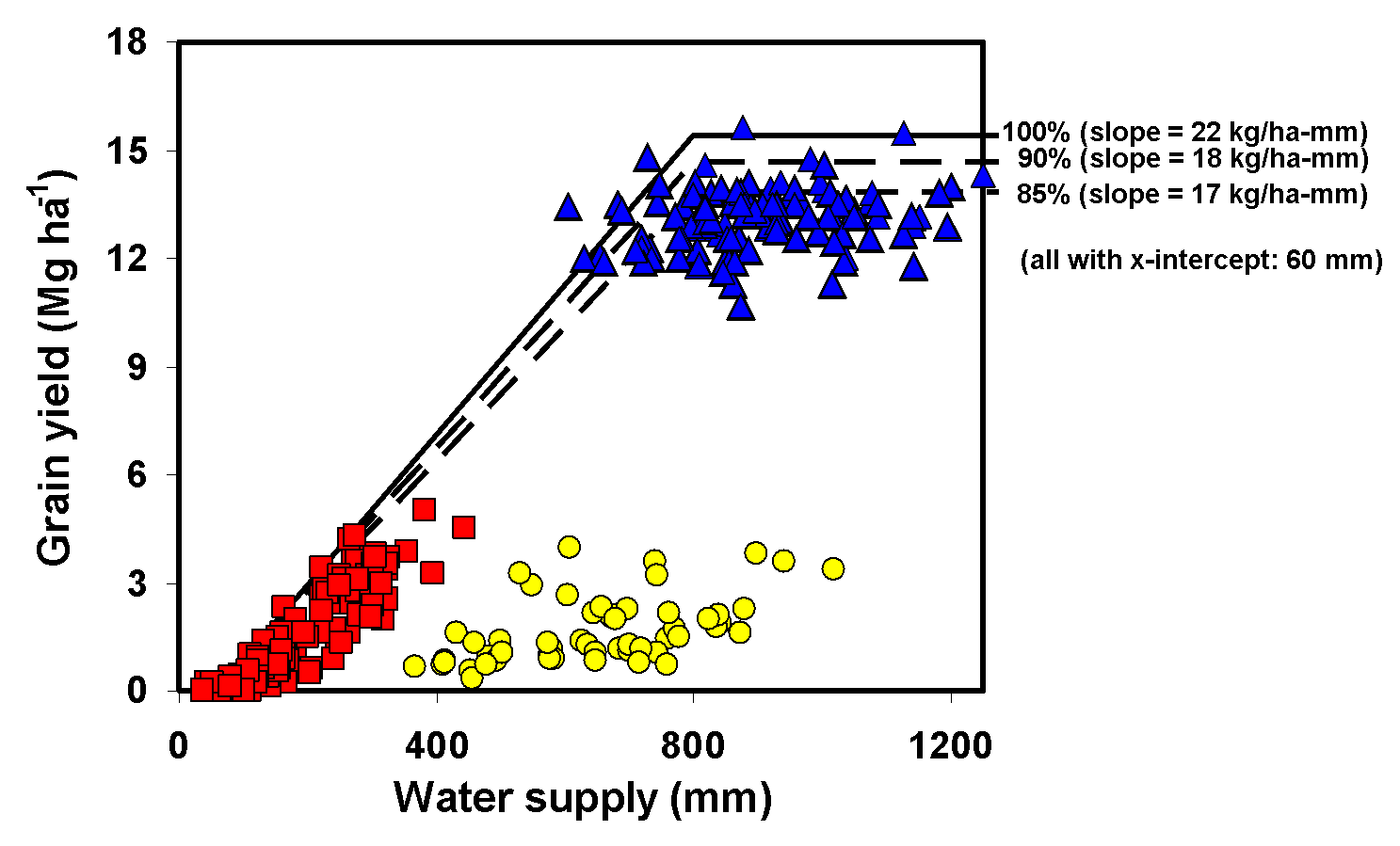
Growth- and yield-related parameters: experiments that can be used for model calibration should have been carried out under optimal growing conditions. Experiments that received sub-optimal management practices should be avoided when calibrating growth- and yield-related model parameters. All data required to run the field-year specific simulations need to be available including: (i) local weather, soil parameters (site-specific data or derived from soil databases), management practices followed by the researchers (planting date, plant population density, cultivar maturity), and initial soil water condition (either measured or estimated through soil water balance). Desirable measured variables for calibration of growth- and yield-related parameters include: aboveground biomass, grain yield, harvest index, and leaf area index. Things to check when screening suitable field experiments data are: yield level, water supply, (discard field experiments in which yields are close to average farmer's yields in low-input, low-yield cropping systems such as SSA Africa), nutrient inputs amount (discard those where nutrient input levels were clearly not adequate for maximum yields), incidence of biotic factors (ideally, the crops should have received prophylactic applications to guarantee no yield reduction due to pests, diseases or weeds), field plots size (don't include yield data from small plots and without replications; preferably do not consider plots smaller than 10 m2 or without replicates), and varieties (experiment should use best locally adapted hybrids or closest best option). Boundary functions relating crop yield to water availability, complemented with expert opinion, can also be used as an aid for model calibration (see Appendix III below). When a boundary function is used, it should be based on a slope relating yield to water supply that is 85% of the frontier boundary function as shown in the figure below (based on Fig 4 from van Ittersum et al, 2013).
APPENDIX III - GUIDELINES FOR MODEL CALIBRATION
The steps in the elaborate model calibration per crop type per zone are the following (with some variation between different models):
- Calibrate phenological development (mainly by changing the model parameters that determine temperature sum requirements for development); Weather data preferences for such calibration follow GYGA methods for yield gap analysis with the following order (first to last preference): (i) actual weather data from within the reference weather station buffer zone in question, (ii) synthetic weather data following GYGA methods for generating such weather data; actual weather data from a location within the same climate zone but outside the RWS buffer, (iii) when no other source of weather data are available, use gridded weather data . For more details about weather data sources and preferences, see GYGA weather data protocols (http://www.yieldgap.org/web/guest/methods-upscaling).
- Verify yield simulations and the cumulative light interception, leaf area index course and total biomass production:
- If simulations are within ±15% of the experimental calibration yield data values or within ±15% of the Yw predicted from the boundary function relating yield with water availability, then stop further calibration.
- If conditions in (1) are not met, the leaf area-related model parameters will be amended within plausible ranges (±20%).
- If after (2), the yield level still deviates more than ±15%, the harvest index (HI) can be modified within ±0.10 of the mean value reported in Table 1 through changing the temperature sum requirements for development before and after flowering and/or assimilate partitioning coefficients.
- Respiration and photosynthesis parameters should be changed only as a last resort if modifications to HI are not sufficient to bring simulated yield within ±15% of experimental calibration yield data. However, if after (3) the yield level still deviates more than ±15%, these parameters can be changed within plausible ranges that are no more than ±10% of published ranges for these parameters.
Table 1. Mean HI for major cereals under optimal growing conditions
| Crop | Plausible mean value |
| Maize | 0.50 |
| (Winter) wheat | 0.50 |
| Rice | 0.50 |
| Millet | 0.30 |
| Sorghum | 0.40 |
APPENDIX IV - HARVEST VERSUS PHYSIOLOGICAL MATURITY DATES
In large-scale, mechanized commercial farming, harvest takes place when grain moisture content reaches a certain level at which mechanical harvest is possible and drying costs are minimized. Therefore, harvest can take place up to 4 weeks after the crop has reached physiological maturity. In these cases, using harvest date as a proxy for physiological maturity can lead to a large bias in the simulated yield. Hence, physiological maturity needs to be retrieved from cultivar total GDD or relative maturity and not from harvest date. If this information is not available, expertise opinion or published data can be used to estimate the GDD from physiological maturity to harvest date. Subsequently, these GDD can be used to derive the physiological maturity date based on the reported harvest date. In small scale, non-mechanized farming (like SSA), harvest occurred around physiological maturity because of (i) pressure to use crop residue for livestock feeding, (ii) risk of insect/diseases/birds/rodents incidence, and (iii) multiple crops per year (Tittonell P., personal communication). Hence, in SSA, reported harvest date can be taken as an estimate of the physiological maturity date. Also, in many cases, crops in SSA are subjected to a very severe terminal drought, therefore, even when harvest date might not coincide with physiological maturity date this mismatch has little effect on the simulated yield.
REFERENCES
Campbell, G.S., and R. Diaz. 1988. Simplified soil–water balance models to predict crop transpiration. p. 15–26. In F.R. Bidinger et al (ed.) Drought research priorities for the dryland tropics. ICRISAT, Pantancheru, India.
Gijsman, AJ, Jagtap, SS, Jones, JW, 2002. Wadding through a swamp of complete confusion: how to choose a method for estimating soil water retention parameters fro crop models. Europ. J. Agronomy 18, 77-106.
Gijsman, AJ, Thornton, PK, Hoogenboom, G. 2007. Using the WISE database to parameterize soil inputs for crop simulation models. Computers and Electronics in Agriculture 56, 85-100.
Ritchie, J.T., Godwin, D.C., Singh, U., 1990. Soil and weather inputs for the IBSNAT crop models. International Benchmark Sites Network for Agrotechnology Transfer (IBSNAT) Project. In: Proceedings of the IBSNAT Symposium: Decision Support System for Agrotechnology Transfer. Part I. Symposium Proceedings, Department of Agronomy and Soil Science, College of Tropical Agriculture and Human Resources, University of Hawaii, Honolulu, Hawaii, Las Vegas, NV, October 16–18, 1989.
Saxton, K.E., Rawls, R.J., 2006. Soil water characteristic estimates by texture and organic matter for hydrologic solutions. Soil Sci. Soc. Am. J. 70, 1569-1578. See also: (http://hydrolab.arsusda.gov/soilwater/Index.htm)
Soltani, A., Sinclair, TR. 2012. Modeling physiology of crop development, growth and yield. CAB, Wallingford, UK. 322 pp.
Tittonell P, Corbeels M, van Wijk MT, Vanlauwe B, Giller KE, 2008. Combining organic and mineral fertilizers for integrated soil fertility management in smallholder farming systems of Kenya—explorations using the crop–soil model FIELD. Agron J 100:1511–1526
van Heemst HDJ, 1988. Plant data values required for simple crop growth simulation models: review and bibliography. Simulation Report CABO-TT Nr. 17. CABO and Department of Theoretical Production Ecology, Agricultural University, Wageningen University.